


The year is 2030, it's been years since the great war between Thanos and The Avengers, you might recall little one, that this war was won by the sacrifice of The Black Widow and the hands of the Iron Man.

Before the war, the king of Wakanda, King T'Challa had decided to open its borders to outsiders starting with the Avengers.

This decision to open Wakanda to the world has brought about a lot of industrial revolution after the war, the fact that Wakanda had some of the most advanced technologies on the planet even before the war made it a center of attraction for techies post-endgame.
Ajoke was one of the techies that migrated to Wakanda after the war, she was originally from Nigeria, she had dropped out of school due to a lack of funds to finance her education. She started learning Data Science on YouTube and she participated in some Kaggle and Zindi competitions to hone her data skills. With time she became a hot cake in the data science community and a company in Wakanda gave her an offer to work as their in-house data scientist here in Wakanda, she accepted the offer and migrated to Wakanda to start working.
Due to the fact that Wakanda is a highly industrial country, the city layout is constructed in such a way that it separates the residential quarters from the industrial regions. Ajoke stays on Road 9, which means she has to go through 9 Kilometers road before she gets to her house. That's a lot of stops so she decided that she'll use Uber instead of taking public transport, Uber has evolved though, they were acquired by The Boring Company 2 years ago, They primarily use tunnels to transport people so you can move at a very high speed. The cost is fair and you even get a personal driver.
Ajoke has to pay the Uber driver 50Wands for initiating the transit and 20Wands for every additional Kilometer, we can put this into an equation so that we can know how much Ajoke has to pay at the end of her trip.
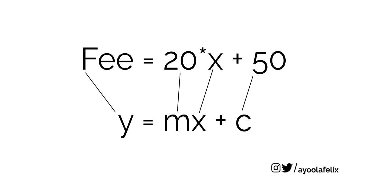
For instance, if she decides to stop at the fifth kilometer to visit a friend.
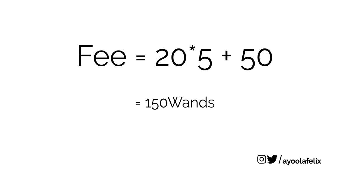
We can write a function that does this automatically in Python and even plots the distance against price for use.
import numpy as np
import matplotlib.pyplot as plt
from matplotlib import style
style.use('fivethirtyeight')
distance = np.array([x for x in range(0,10)], dtype = np.float64)
price = np.array([20*x + 50 for x in range(0, 10)], dtype= np.float64)
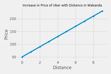
plt.scatter(distance, price)
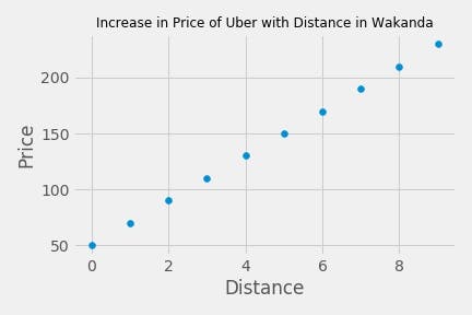
plt.title('Increase in Price of Uber with Distance in Wakanda', fontsize = 12)
plt.xlabel('Distance')
plt.ylabel('Price')
plt.show()
You should have this plot
In the real world, your m and b will not be known before, you'll have to calculate it but it's not hard just one simple function but first we must know the formula or calculating the slope(m) and the intercept(b).
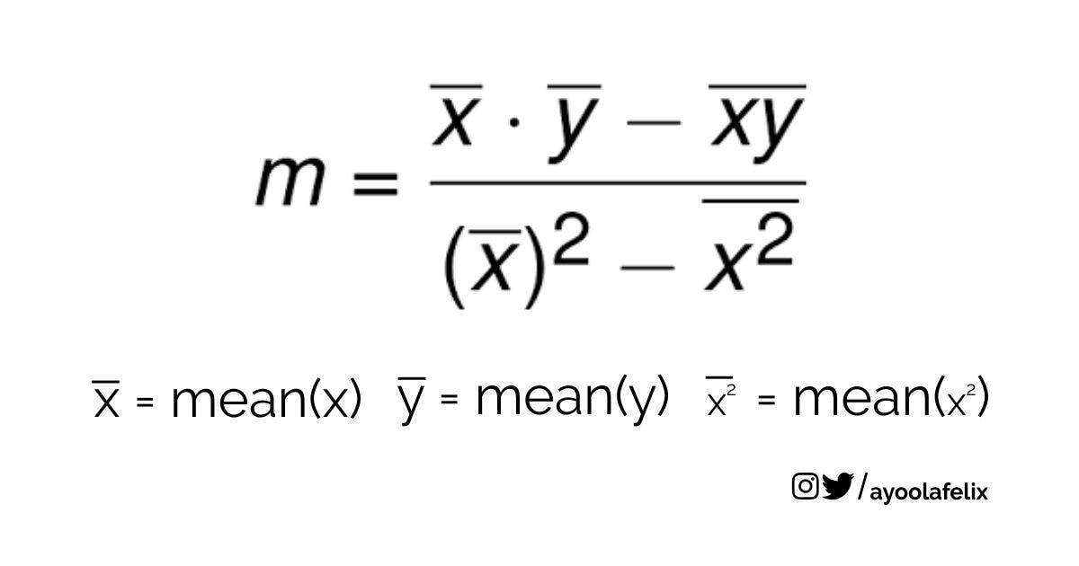
def best_fit_slope_and_intercept(x, y):
m = (((mean(x) * mean(y)) - mean(x * y))
/ ((mean(x) ** 2) - mean(x ** 2)))
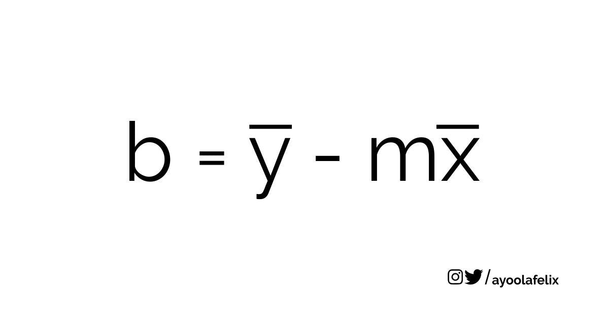
b = mean(y) - m* mean(x)
return m, b
Applying this to Ajoke's use case, we use the gradient(m) and slope(b) we get from our function to calculate the price for each distance, then we plot the distance against the corresponding price to get our regression line.
import numpy as np
import matplotlib.pyplot as plt
from matplotlib import style

style.use('fivethirtyeight')

distance = np.array([x for x in range(0,10)], dtype = np.float64)
price = np.array([20*x + 50 for x in range(0, 10)], dtype= np.float64)

def best_fit_slope_and_intercept(distance, price):
    m = (((mean(distance) * mean(price)) - mean(distance * price))
        / ((mean(distance) ** 2) - mean(distance ** 2)))
    b = mean(price) - m* mean(distance)
    return m, b

m, b = best_fit_slope_and_intercept(distance, price)
regression_line = [(m*x) + b for x in distance]

plt.plot(distance, regression_line)
plt.scatter(distance, price)
plt.title('Increase in Price of Uber with Distance in Wakanda', fontsize = 12)
plt.xlabel('Distance')
plt.ylabel('Price')
plt.show()
You should get something like this
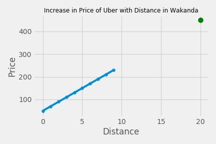
Now you've plotted a regression line, with this regression line you can predict the price for let's say Ajoke decides to go 20 Kilometers to visit a friend since we know m and b
import numpy as np
import matplotlib.pyplot as plt
from matplotlib import style

style.use('fivethirtyeight')

distance = np.array([x for x in range(0,10)], dtype = np.float64)
price = np.array([20*x + 50 for x in range(0, 10)], dtype= np.float64)

def best_fit_slope_and_intercept(distance, price):
    m = (((mean(distance) * mean(price)) - mean(distance * price))
        / ((mean(distance) ** 2) - mean(distance ** 2)))
    b = mean(price) - m* mean(distance)
    return m, b

m, b = best_fit_slope_and_intercept(distance, price)

predict_distance = 20
predict_price = (m*predict_distance) + b
print(predict_price)
Running this code, we should get 450Wands as the answer, while this is correct and very accurate, in the real world, data isn't usually this clean so you might end up with something messy and not 100% accurate but today you've learned what linear regression is and how to use it. Let's recap in case you want to try this with a messy data.
- Calculate m and b
- Use these values to predict your y by using y = m*x + c
Everything we've done can be complied into this code
import numpy as np
import matplotlib.pyplot as plt
from matplotlib import style

style.use('fivethirtyeight')

distance = np.array([x for x in range(0,10)], dtype = np.float64)
price = np.array([20*x + 50 for x in range(0, 10)], dtype= np.float64)

def best_fit_slope_and_intercept(distance, price):
    m = (((mean(distance) * mean(price)) - mean(distance * price))
        / ((mean(distance) ** 2) - mean(distance ** 2)))
    b = mean(price) - m* mean(distance)
    return m, b

m, b = best_fit_slope_and_intercept(distance, price)
regression_line = [(m*x) + b for x in distance]

predict_distance = 20
predict_price = (m*predict_distance) + b
print(predict_price)

plt.scatter(predict_distance , predict_price, s = 100, color = 'g')

plt.plot(distance, regression_line)
plt.scatter(distance, price)
plt.title('Increase in Price of Uber with Distance in Wakanda', fontsize = 12)
plt.xlabel('Distance')
plt.ylabel('Price')
plt.show()
On this plot, you'll see a new dot for the 20km and the price it corresponds to.
I hope this article begins your journey into understanding that mathematics for Data Science can be simplified and understood.
Thanks for reading, you can hit me up on Twitter [Felix Ayoola].